Archive | IMU RSS feed for this section

IMU Acceleration, Gyro, & Magnetometer Calibration

In an effort to produce reliable quantitative angles of tilt and roll of the IMU module, it is necessary to calibrate all 9-axis vectors. Acceleration, gyroscope, and magnetometer are together calibrated together as a single system where reliable calculation and measurement of tilt and roll functions become achievable. In this post, an explanation of how the calibration is done to include visual verification leads to the successful application of tilt and roll measurement as demonstrated. To get an accurate approximation of tilt and roll measurements, calibration of all vectors is necessary. Effectively, this project provides a way to obtain tilt in two different directions using the BNO055 IMU module.

Screen Capture 1 – Calibration data readings that correspond to visual plotting of each combined level to 3,3,3,3. See legend in image that indicates varying levels before stability at achieved calibration.

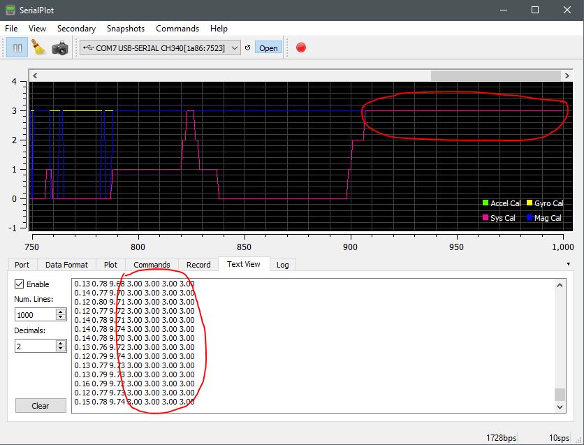
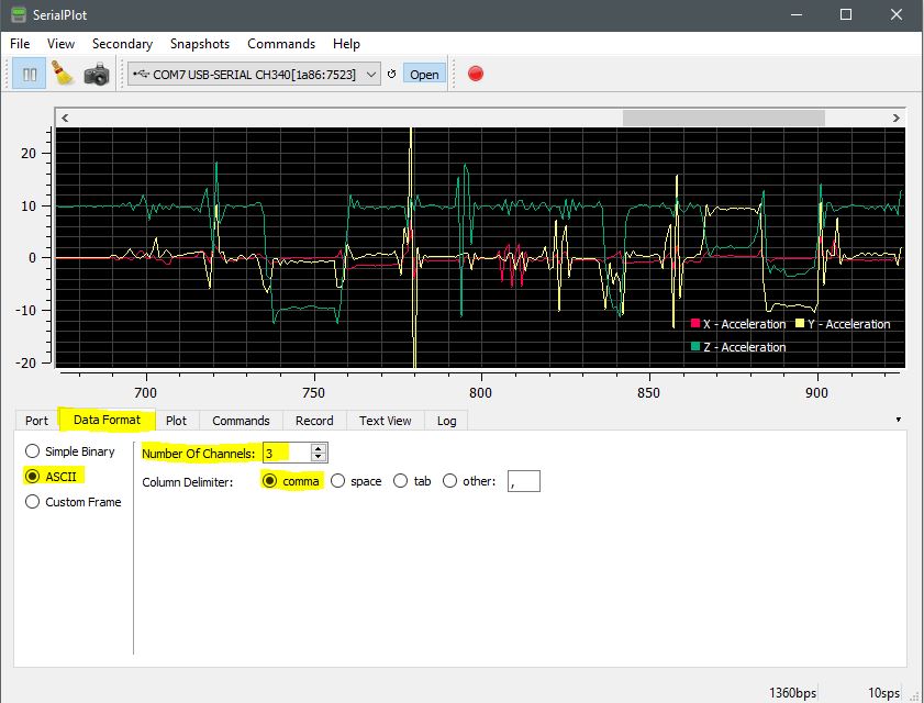
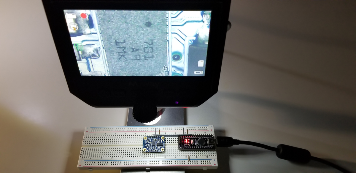
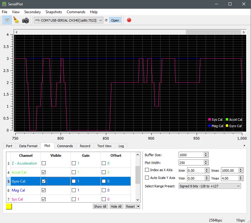
All four calibration categories must register in the data acquisition stream as 3,3,3,3. Three-axis together as three for each category to include the system which is the combined fused total of the three. When first running the IMU module, or after reset, the data readings will appear at 0 until all four settles into position as 3. To get each to settle (accel, gyro, mag, and sys), it is necessary to physically rotate the IMU module. Move the IMU around in a figure-8 motion and watch for the data readings to rise from 0 to 3.


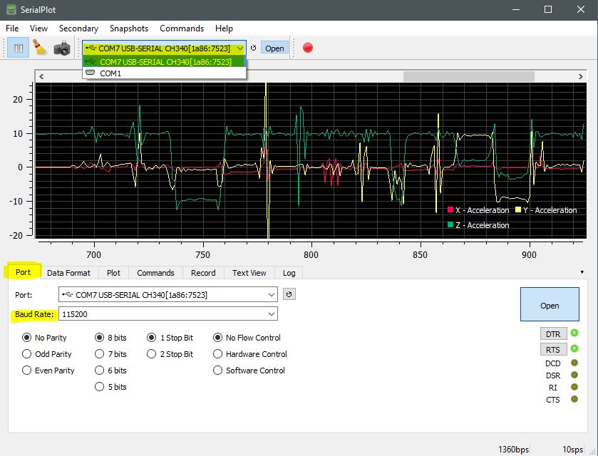
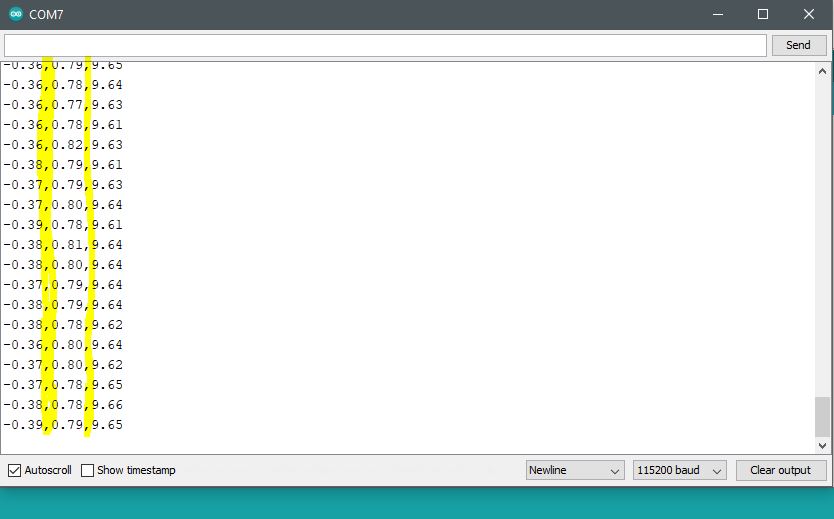
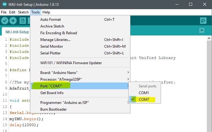
Sometimes the numbers among all four columns will drop below three, but eventually, they will all four level-out at 3. At times a single column number will not get to three and can appear stubborn. So it is important to hold the IMU in 45-degree roll, tilt, and yaw increments for a few seconds each. That is usually the most effective approach to get all four vectors to align at 3,3,3,3. It is always important to keep the IMU unit away from sources of magnetism, or motors, or sources of EMI that could adversely affect calibration, or an ability to achieve calibration. Keep the IMU away from sources of EMI during calibration while watching for acc, gyro, mag, and sys levels visually plotted and quantitatively acquired in the data readings (see Text View tab).

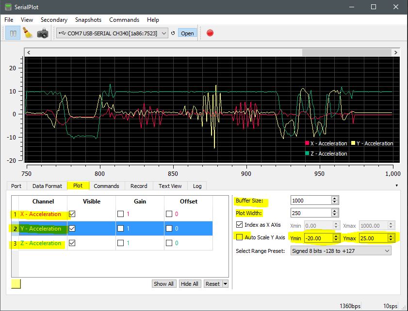
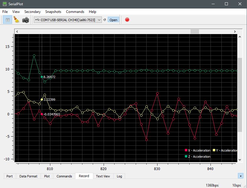
When all four vector categories are in alignment, it then becomes possible to run tilt and roll tests to obtain reliable confidence in tilt and toll angles of measurement. Notice that the calibration legend is set by category within the Plot tab. Simply double click the Channel name to rename it to a label that is suitable. It is also necessary to set the Auto Scale Y-Axis to a readable number between 0 and 4. That way it is easier to see the variability in calibration by visual recognition. Otherwise, you rely solely on the 3,3,3,3, quantitative measures within the Text View tab as depicted in Screen Capture 1 above.

Screen Capture 2 – Enable calibration channels and set Y Axis Scale for readability of data acquisition.

To monitor tilt and roll it will be necessary to deselect the acceleration, gyro, magnetometer, and system channels to disable the plot and legend. You may want to do this as more serial.print lines in code to display tilt and roll angles will plot separately as additional channels.

Screen Capture 3 – Deselect calibration channels and reset the Y-axis scale for angular data readings. Setting -90 to 90 degrees is better, but for a full range example -180 to 180 is demonstrated here to indicate wide, but accurate variability for the best approximation.

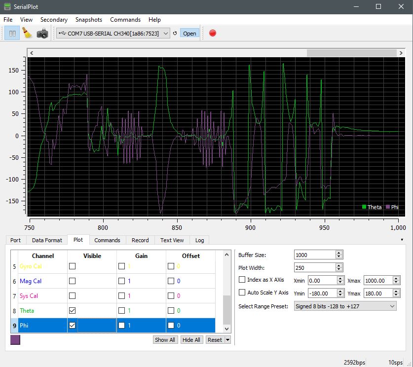
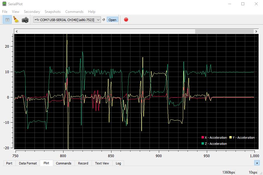
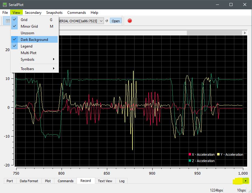
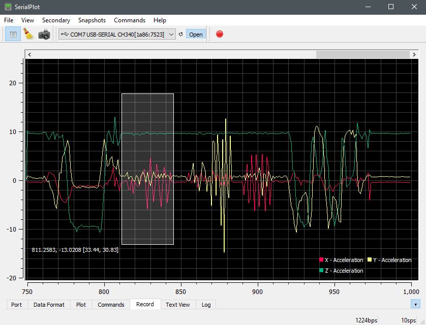
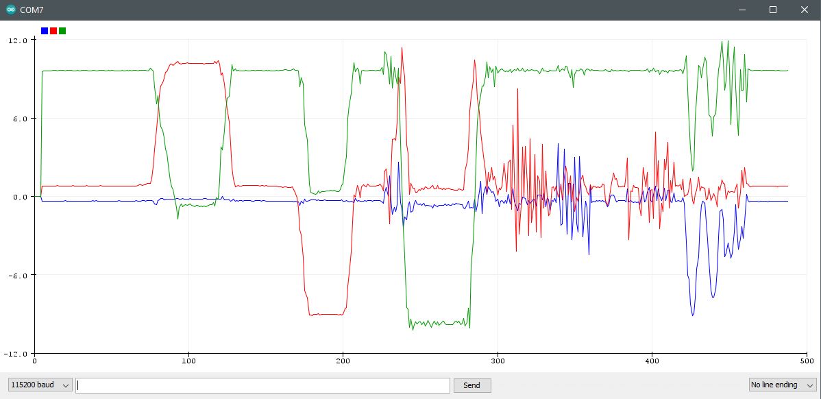
Once calibration is set and the plot graph is ready to display the angular channels (theta and phi), you can physically tilt and roll the IMU module to get positive and negative angles of movement and position. The calculated and plotted serial data that represents rotation along the y-axis is the name theta in this example. It represents a physical tilt action from up (positive) to down (negative) angles of movement. Conversely, the roll motion is physical rotation along the x-axis, so named phi in this example. Physical rotation along the x-axis right (positive) and left (negative) also get plotted and acquired within the data readings within the Text View tab.

Screen Capture 4 – Tilt and roll measurements (+/- degrees of rotation) of both theta and phi with a fully calibrated IMU module.

As written about before, acceleration, gyro, and magnetometer, as separate categories, each has 3-axis degrees of freedom. Where all three together produce a total of 9-degrees of freedom. So, with each category, a unity of 3 for each gives us confidence that they are all together, yet separately, calibrated.

Project Review:

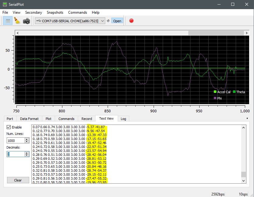
A physical demonstration is captured here both visually and quantitatively. As roll and tilt movement is applied to the IMU module, corresponding positive and negative angles of change become plotted and logged for quantitative analysis.


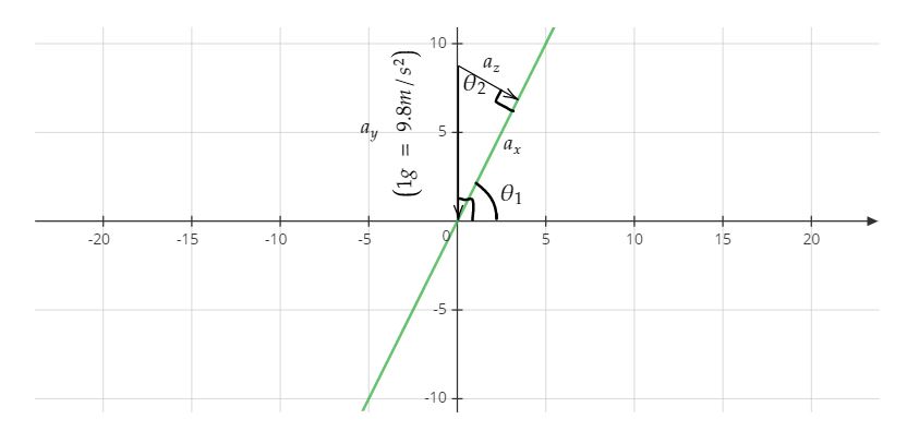
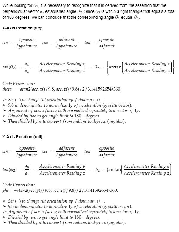
Tilt & Roll Calculations:
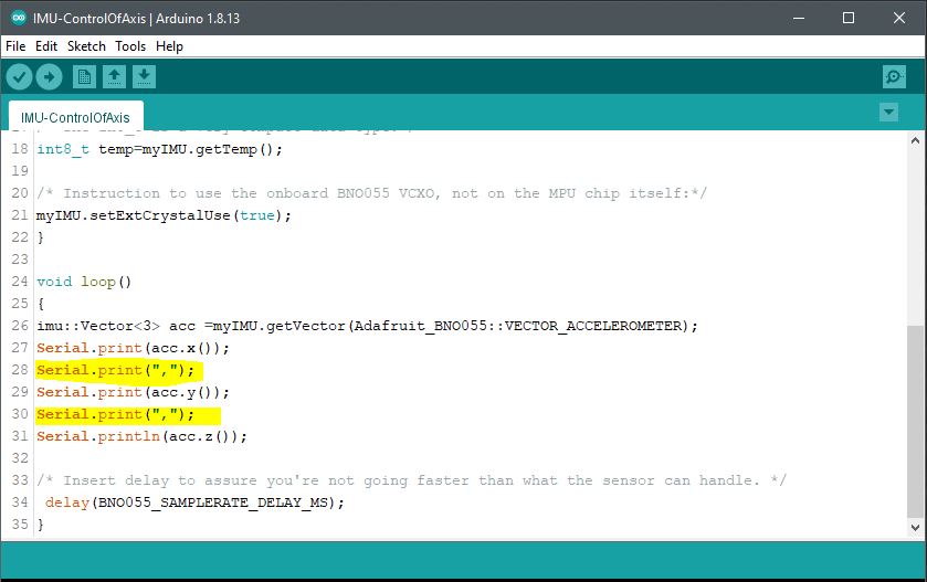
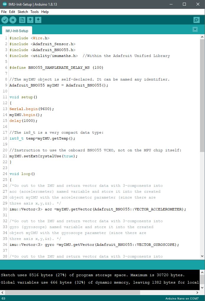
Code Example:

#include <Wire.h>
#include <Adafruit_Sensor.h>
#include <Adafruit_BNO055.h>
#include <utility/imumaths.h> //Within the Adafruit Unified Library
#include <math.h> //Permits inverse tangent function below

float theta;
float phi;

#define BNO055_SAMPLERate_DELAY_MS (100)

/* The myIMU object is self-declared. It can be named any identifier.*/
Adafruit_BNO055 myIMU = Adafruit_BNO055();

void setup()
{
Serial.begin(115200);
myIMU.begin();
delay(1000);

/* The in8_t is a very compact data type:*/
int8_t temp=myIMU.getTemp();

/* Instruction to use the onboard BNO055 VCXO, not on the MPU chip itself:*/
myIMU.setExtCrystalUse(true);
}

void loop()
{

uint8_t system=0, gyro=0, accel=0, mg=0; /*Byte sized variable data type */
myIMU.getCalibration(&system, &gyro, &accel, &mg);
imu::Vector<3> acc =myIMU.getVector(Adafruit_BNO055::VECTOR_ACCELEROMETER);

/*A calculated approximation of tilt (inverse tangent (ax/9.8) divided by (az/9.8)).
The 9.8 denominator in each term is to normalize the vector to 1-g for each variable.
Then dividing by 2 and 3.14 (pi) converts the measurement units to degrees.*/

theta=-atan2(acc.x()/9.8,acc.z()/9.8)/2/3.141592654*360;
phi=-atan2(acc.y()/9.8,acc.z()/9.8)/2/3.141592654*360;


Serial.print(acc.x()/9.8);
Serial.print(“,”);
Serial.print(acc.y()/9.8);
Serial.print(“,”);
Serial.print(acc.z()/9.8);
Serial.print(“,”);
Serial.print(accel);
Serial.print(“,”);
Serial.print(gyro);
Serial.print(“,”);
Serial.print(mg);
Serial.print(“,”);
Serial.print(system);
Serial.print(“,”);
Serial.print(theta);
Serial.print(“,”);
Serial.println(phi);

/* Insert delay to assure you’re not going faster than what the sensor can handle. */
delay(BNO055_SAMPLERATE_DELAY_MS);
}


IMU Data Serial Plotter Setup and Configuration

Similar to the serial plotter on the Arduino Sketch IDE, there is a useful real-time serial plotter application at the Hackaday site. It is free and it offers configuration options that add to the utility of data tracking, measurement, and analysis. The application provides for scroll, zoom, cursor, channel selections, and color options that ease how visually parsed data is presented and managed. There is a range of capabilities with the utility that makes it a better way to go over the Sketch IDE data plotter.

Example data acquisition from plotted data points over time.

While the link provided gives a way to download and install the latest data plotter version, this post makes use of the following file:

Once the utility is installed and running, there are configuration options I use to monitor the IMU serial data streams. Specifically, it is necessary to select the available COM port connected to the USB port on the Arduino host of the IMU module. Once that is done, the Baud Rate selected within the application’s Port tab must match the baud rate declared in the void setup() segment of your Arduino code. In this example, my declaration is Serial.begin(115200), so the baud rate selection must be 115200). The standard serial handshaking configurations apply as 8-bit, 1 stop bit, no parity, and no flow control.

It is important that the Arduino Sketch serial plotter application isn’t running as it will present a conflict with this utility.

Screen Capture 1 – Port selection and baud rate.

Next is formatting the data according to how the vector data acquisition code is written as an ASCII data type and for proper delimiting. Since the comma it used for data capture, that option is selected.

Screen Capture 2 – Data type and delimiter settings
Screen Capture 3 – Program code that declares the comma.
Screen Capture 4 – Sketch IDE Serial Monitor that streams acquired data with comma separation / delimiting.

While the three acceleration vectors x, y, z automatically populated according to the number of channels in screen capture two (2) above. To add more channels (vectors), simply increase the quantity from the data format tab. The buffer size setting corresponds to the vector data held in memory and gets displayed along the x-axis in the plotter graph. Setting the plot width to a narrow data window increases the plotted data acquisition rate from right to left. The scale axis settings simply correspond to the amplitude of inflections observed in the data.

Screen Capture 5 – Data plotter configuration. Double-click each channel field within the Plot tab to name the data as desired for legend placement and identification.

The other four tabs have less relevance in the set up here, but they are useful to record and monitor data as an output to acquired data. To further explore settings for visual quality and precision, experiment with the menu options to get your desired layout and format.

Screen Capture 6 – Layout and graphical format options for visual quality.
Screen Capture 7 – Zoom window by cursor selection to expand and view further into data points. Right click within the pane to reset full view.
Screen Capture 8 – Zoomed in view of acquired data segment.

Project Review:


BNO055 IMU 9-Axis DOF Acceleration Analysis

In an effort to further delve into the inner workings of the BNO055 accelerometer and its functions, the serial plotter was applied to the project. To better understand how the produced data is rendered over the I2C SDA/SCL connection to the Nano, the data is translated by the plotter into a visual char as presented below. The gyro and magneto functions of the IMU are not included in this review to get a better depth of understanding around the module’s capabilities.

The amount of capacitive charge capacity within a capacitor. The permittivity of an insulator (ε) describes the insulator’s resistance to the creation of an electric field and is equal to 8.85×10⁻¹² Farads per meter for an air-gap capacitor.

The three-axis of acceleration is plotted over time as a function of latitude movement (x-axis), longitude movement (y-axis), and vertical movement (z-axis). As the IMU module is moved and oriented to different positions, the sensor interprets that activity by measurement of differences in charge. Specifically, internally charged surfaces are separated by differences in area and distance to vary a combined capacitive charge. That change in charge, as measured, corresponds to the difference in acceleration since internal plate movement varies in all three directions.

In the photo here, imagine that a lower plate is moving up and down, back and forth through its comb structure. The surface area for each direction of movement brings about a difference in capacitive charge where that becomes interpreted as acceleration. The substrate below the comb structure consists of a surface area that corresponds to the z-axis charge that is tracked for changes in vertical acceleration. The lattice framed structure is suspended by springs to assure continuous and precise movement in any direction within defined limits.

It is again useful to recognize that the amount of charge present within the capacitor, or capacitive body, is determined by the surface area and distance between two charged plates. Reduce the surface area between the two plates, and the total capacitive charge is reduced. Increase the distance between the two plates and the capacitive charge is reduced. This simplified explanation does not take into account any dielectric properties that exist among different types of capacitors.

Red: X-axis latitude acceleration. Blue: Y-axis longitude acceleration. Green: Z-axis vertical. Notice that the green plot is tracking at
9.8m/s2 since that is the acceleration of gravity present at the IMU module. The -9.8m/s2 reading is with the IMU inverted with the internal
micro-electro-mechanical (MEM) structure pulled down by gravity.

Project Schematic:

The same basic connections are in place as before in the prior set up project. The key I2C communication connections between the modules remain in place to transfer clock and data for integration and processing. Both modules share the same ground and 5V VCC.

Project Review:

As demonstrated in this video, the IMU module’s data plot extends across time as the acceleration tests are carried out. As the IMU module is moved to different positions and orientations, observe the corresponding changes in plotted graphical data.


Code Example:

#include <Wire.h>
#include <Adafruit_Sensor.h>
#include <Adafruit_BNO055.h>

/* Within the Adafruit Unified Library*/
#include <utility/imumaths.h>

#define BNO055_SAMPLERATE_DELAY_MS (100)

/* The myIMU object is self-declared. It can be named any identifier.*/
Adafruit_BNO055 myIMU = Adafruit_BNO055();

void setup()
{
Serial.begin(115200);
myIMU.begin();
delay(1000);

/* The in8_t is a very compact data type:*/
int8_t temp=myIMU.getTemp();

/* Instruction to use the onboard BNO055 VCXO, not on the MPU chip itself:*/
myIMU.setExtCrystalUse(true);
}

void loop()
{
imu::Vector<3> acc =myIMU.getVector(Adafruit_BNO055::VECTOR_ACCELEROMETER);
Serial.print(acc.x());
Serial.print(“,”);
Serial.print(acc.y());
Serial.print(“,”);
Serial.println(acc.z());

/* Insert delay to assure you’re not going faster than what the sensor can handle. */
delay(BNO055_SAMPLERATE_DELAY_MS);
}


BNO055 IMU 9-Axis DOF Hardware & Software Setup

Once initial hardware is in place, it is necessary to gather the libraries to run the software and get connectivity and begin gathering the Arduino unit and the BNO055 IMU Fusion module data. In this setup, various libraries are needed to run the code as it becomes developed in this post and further along among projects.

Project Schematic:

The physical build of the IMU assembly is very simple. Wiring between the IMU module and the Arduino Nano is as illustrated in the schematic below.

BNO055 Module:

The pins on the BNO055 are laterally interspersed by function. Namely, Power, I2C, and Utility. With VIN, 3VO, and Ground as the power input pins, the SDA (serial-data) and SCL (serial clock) are the I2C pins, and finally a mix of addressing, interrupt and mode pins (RST, INT, ADR, & PS0/PS1).

BNO055 Pinout:

PinNameDescription
1VIN3.3-5.0V power supply input
23VO3.3V output from the onboard linear voltage regulator, you can draw up to about 50mA.
3GNDThe common/GND pin for power and logic.
4SDAI2C data pin, connect to your microcontroller’s I2C data line. This pin can be used with 3V or 5V logic, and there’s a 10K pullup on this pin.
5SCLI2C data pin, connect to your microcontroller’s I2C data line. This pin can be used with 3V or 5V logic, and there’s a 10K pullup on this pin.
6RSTHardware reset pin. Set this pin low then high to cause a reset on the sensor. This pin is 5V safe.
7ADRSet this pin high to change the default I2C address for the BNO055 if you need to connect two ICs on the same I2C bus. The default address is 0x28. If this pin is connected to 3V, the address will be 0x29.
8INTThe HW interrupt output pin, which can be configured to generate an interrupt signal when certain events occur like movement detected by the accelerometer, etc. (not currently supported in the Adafruit library, but the chip and HW are capable of generating this signal). The voltage level out is 3V.
9PS1This pin can be used to change the mode of the device (it can also do HID-I2C and UART) and also is provided in case Bosch provides a firmware update at some point for the ARM Cortex M0 MCU inside the sensor. Should normally be left unconnected.
10PS0This pin can be used to change the mode of the device (it can also do HID-I2C and UART) and also is provided in case Bosch provides a firmware update at some point for the ARM Cortex M0 MCU inside the sensor. Should normally be left unconnected.

Project Review:

The physical movement of the IMU along the various degrees of freedom (DOF), produces vector data as demonstrated in this video. A before and after comparison of the data by a change of position indicates changes in the acceleration and gyroscope to validate positive and negative orientation.


Arduino IDE:

Arduino Libraries:

Arduino Serial Monitor:

Once a suitable serial COM port is selected from the tools menu, access to the Serial monitor is made available to call for its use in the setup code of the program (under void setup()) function as Serial.begin([baudrate]).

Select Suitable COM Port

Select Serial Monitor

View Serial Monitor for Vector Data

Code Example:

#include <Wire.h>
#include <Adafruit_Sensor.h>
#include <Adafruit_BNO055.h>
#include <utility/imumaths.h> //Within the Adafruit Unified Library

//The myIMU object is self-declared. It can be named any identifier.
Adafruit_BNO055 myIMU = Adafruit_BNO055();

void setup()
{
Serial.begin(9600);
myIMU.begin();
delay(1000);

//The in8_t is a very compact data type:
int8_t temp=myIMU.getTemp();

//Instruction to use the onboard BNO055 VCXO, not on the MPU chip itself:
myIMU.setExtCrystalUse(true);
}

void loop()
{
/*Go out to the IMU and return vector data with 3-components into
acc (accelerometer) named variable and store it into the created
object myIMU with the accelerometer parameter (since there are
three-axis x,y,&z). */

imu::Vector<3> acc =myIMU.getVector(Adafruit_BNO055::VECTOR_ACCELEROMETER);

/*Go out to the IMU and return vector data with 3-components into
gyro (gyroscope) named variable and store it into the created
object myIMU with the gyroscope parameter (since there are
three-axis x,y,&z). */

imu::Vector<3> gyro =myIMU.getVector(Adafruit_BNO055::VECTOR_GYROSCOPE);

/*Go out to the IMU and return vector data with 3-components into mag (magnetometer) named variable and store it into the created object myIMU with the magnetometer parameter (since there are three-axis x,y,&z). */

imu::Vector<3> mag =myIMU.getVector(Adafruit_BNO055::VECTOR_MAGNETOMETER);

Serial.print(“Acceleration X-Vector: “);
Serial.println(acc.x());
Serial.print(“Acceleration Y-Vector: “);
Serial.println(acc.y());
Serial.print(“Acceleration Z-Vector: “);
Serial.println(acc.z());
Serial.println(” “);
Serial.print(“Gyroscope X-Vector: “);
Serial.println(gyro.x());
Serial.print(“Gyroscope Y-Vector: “);
Serial.println(gyro.y());
Serial.print(“Gyroscope Z-Vector: “);
Serial.println(gyro.z());
Serial.println(” “);
Serial.print(“Magnetometer X-Vector: “);
Serial.println(mag.x());
Serial.print(“Magnetometer Y-Vector: “);
Serial.println(mag.y());
Serial.print(“Magnetometer Z-Vector: “);
Serial.println(mag.z());
Serial.println(” “);

/* Insert delay to assure you’re not going faster than what the sensor can handle. */
delay(BNO055_SAMPLERATE_DELAY_MS);
}