Archive | Engineering RSS feed for this section

Battery Powered Nano Development Module

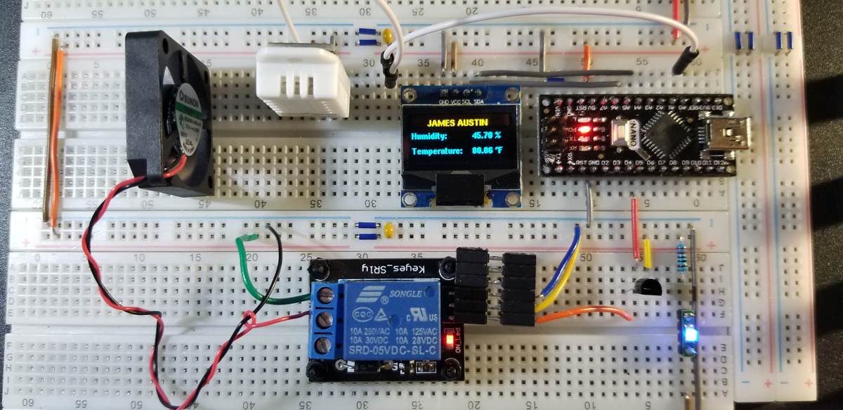
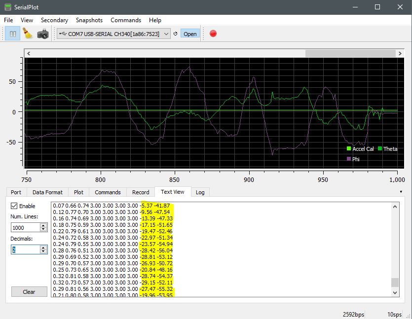
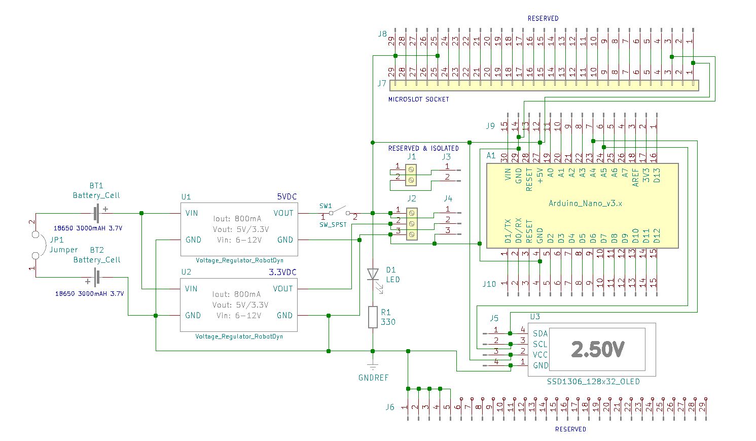
While experimenting with a 128×32 OLED as a voltage meter, it becomes apparent that the display and its associated Arduino SBC provide a pretty good way to set them together on a printed circuit board as a fixed platform for added development. In addition to a pair of 18650 batteries (2S1P), a 5VDC and 3.3VDC regulator are together fed by a range of 8.4VDC to 6VDC (fully discharged). So the Arduino and its display in this project are set to a permanent display on a printed circuit board with a power switch and separate breakout connections.

The point of the build is to set up a module that supports repeatable attachments such as sensors, or micro-slot modules developed separately. Without having to disassemble or configure system components, its power supply, regulators, display, interface terminals, and breadboard connections, all remain the same. This is to facilitate the placement and programming of the same hardware across various projects without much concern for what attachments are made (or declared and configured in code).

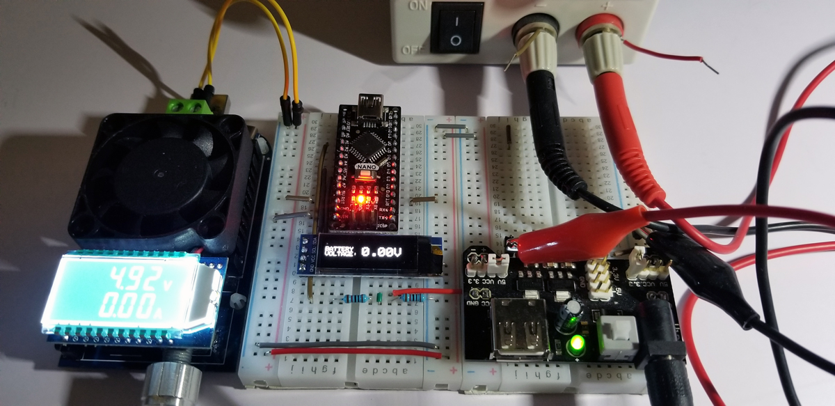
While setting up the breadboard to test viability, it became apparent that the supply voltage at the Arduino had to be regulated. Due to a range of possible loading conditions, the supply voltage could sag or drop to adversely affect performance or minimum operating conditions.
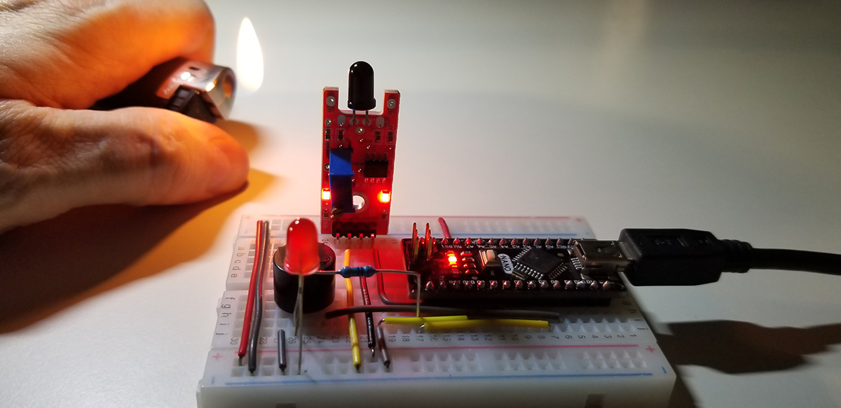
Test & Validation:

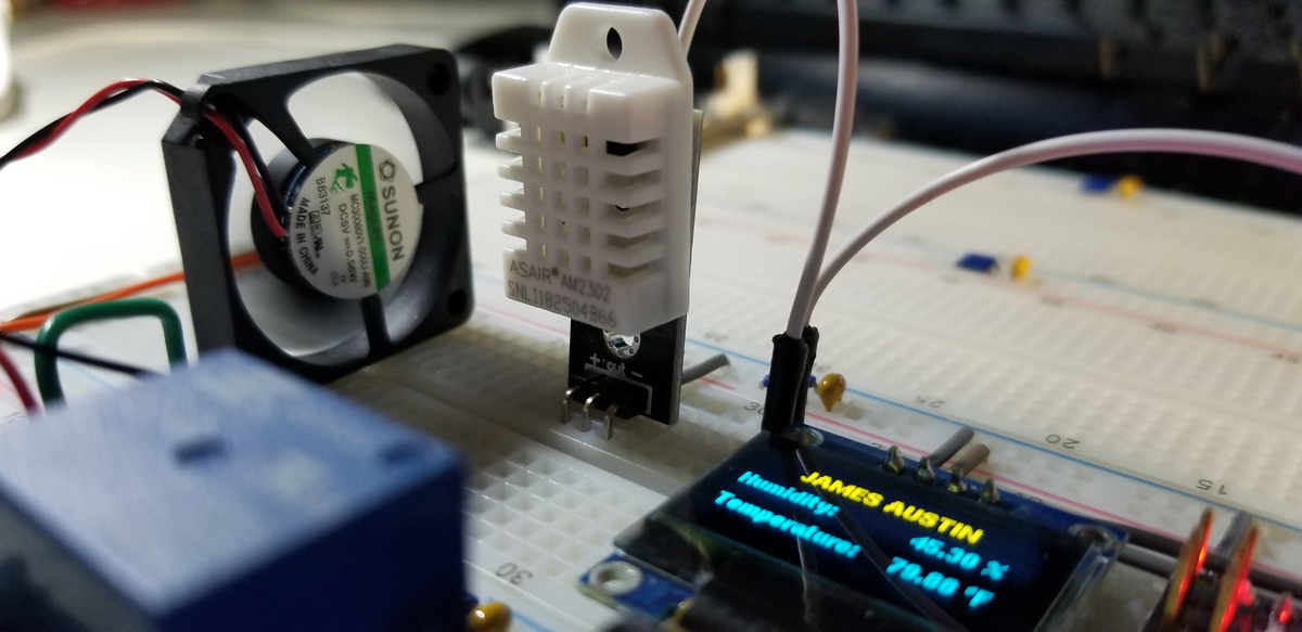
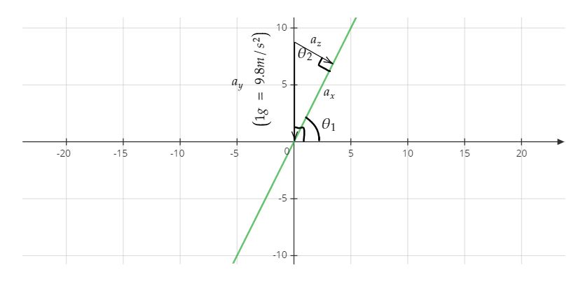
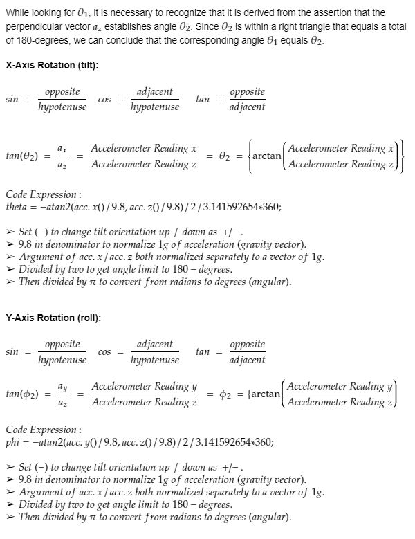
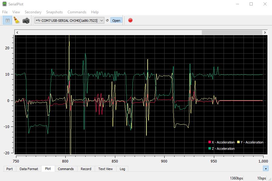
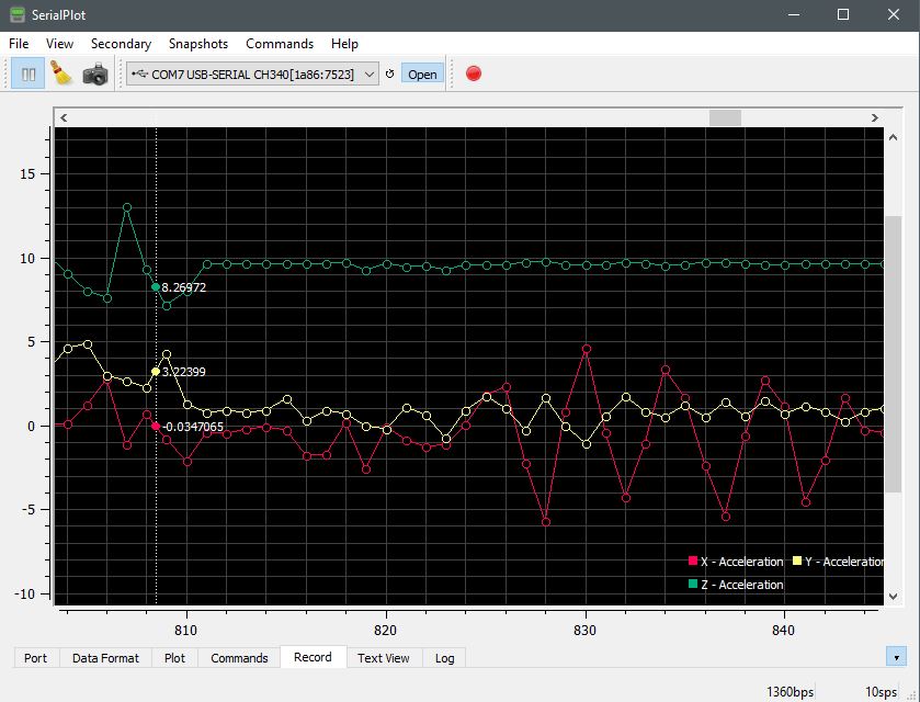
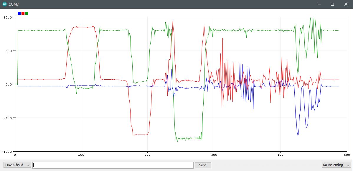
In this video, the supply voltage is from an outside wall adapter (measured at about 4.92VDC unregulated). The voltage measurement on the 128×32 OLED is the two battery scenarios (2x AAA and 1x 18650). The instrument measurements are simply to confirm the Arduino measurements presented at the OLED. The code within the Arduino Nano module had to specify a 4.92VDC reference to get an accurate target reading. So it became apparent just in this experiment, the source voltage was necessary to regulate to assure a steady reference.
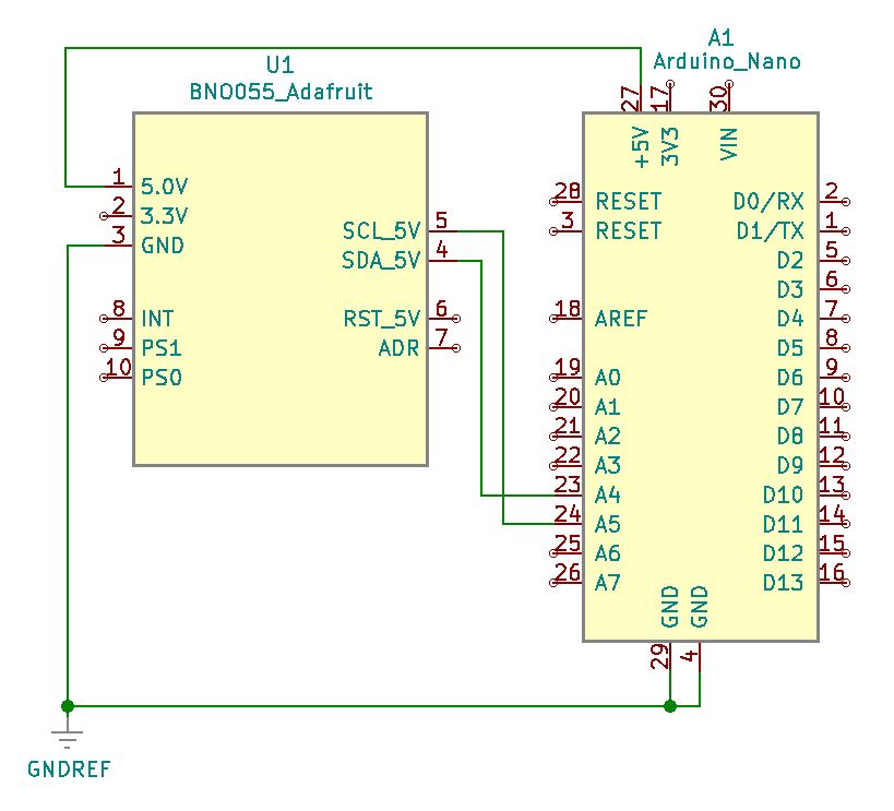
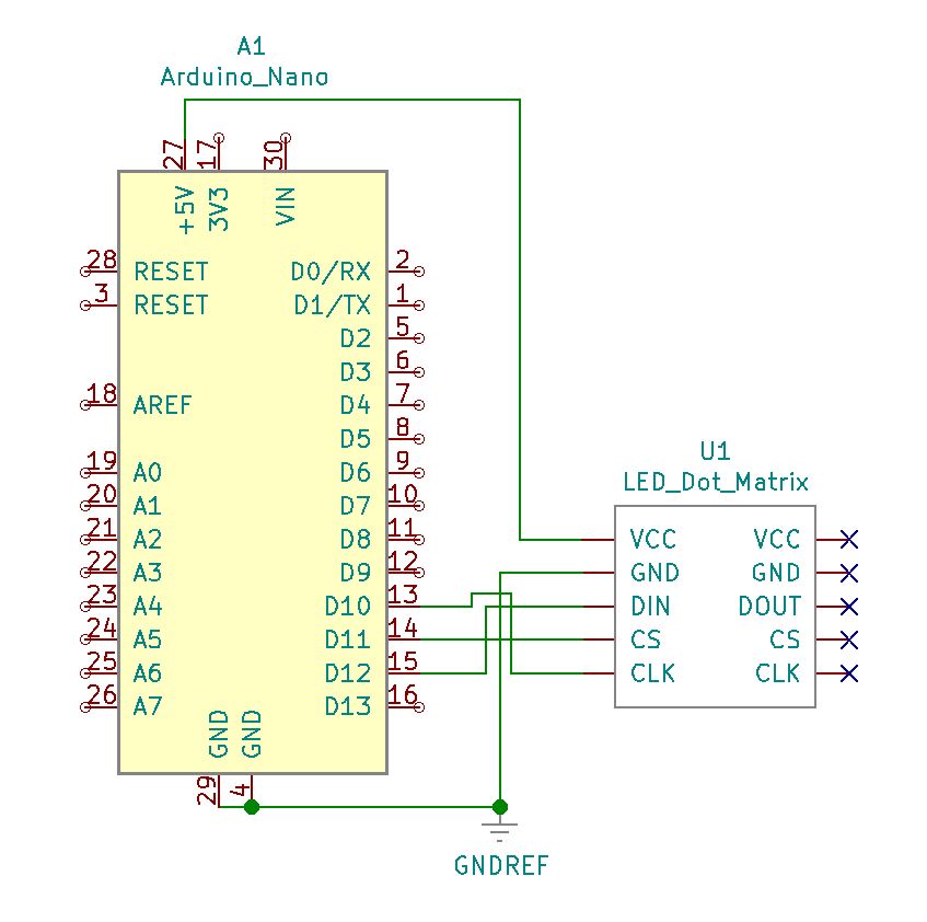
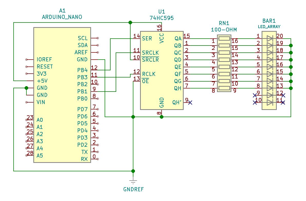
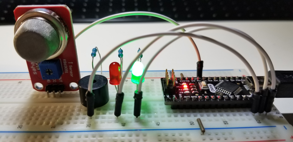
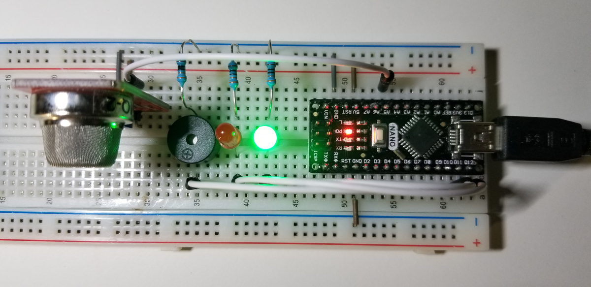
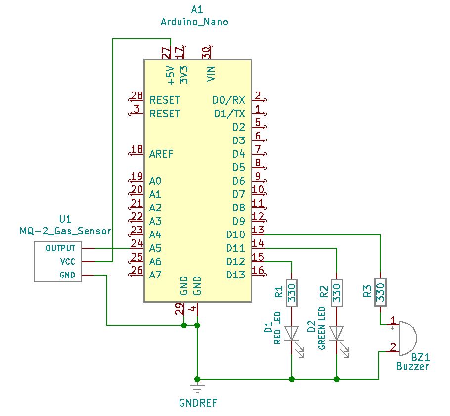
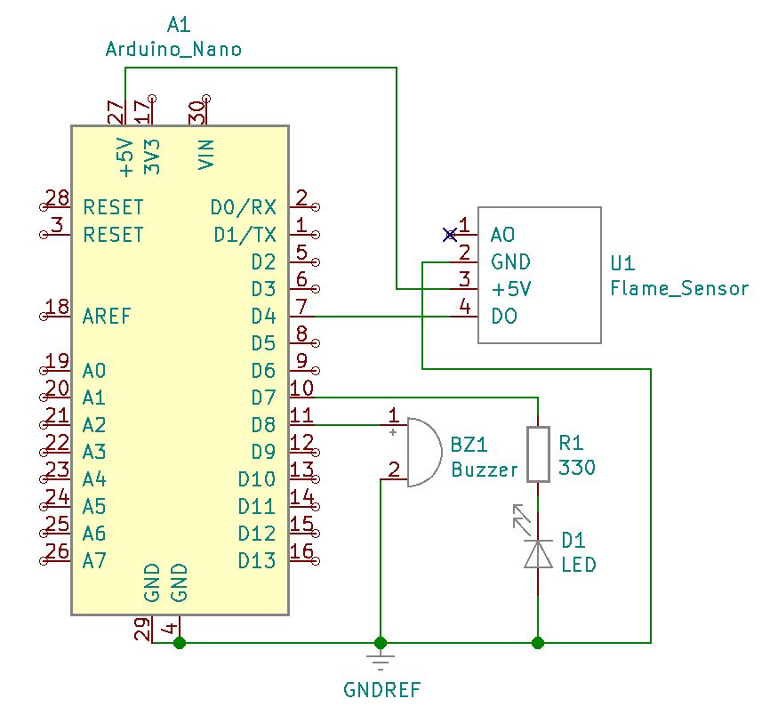

Project Schematic:

Common connections frequently repeated among project various projects include a power supply, regulator(s), a display, and connections such as terminal blocks or pin headers. All elements set together provide an efficient way to develop separate system attachments to limit efforts around new hardware or overall code development.
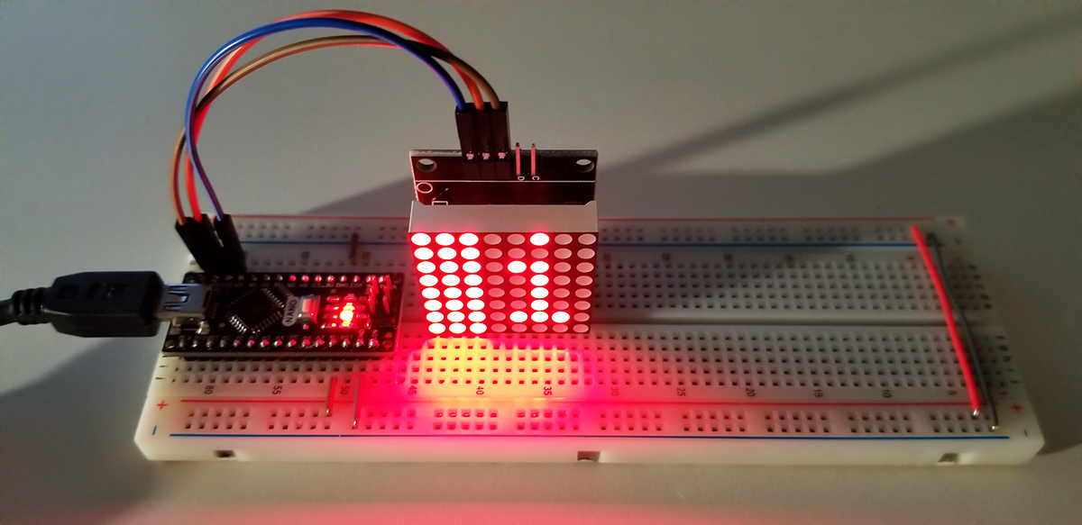
Project Build:

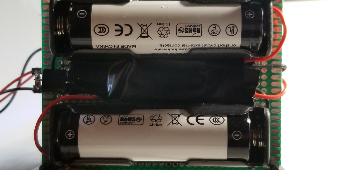
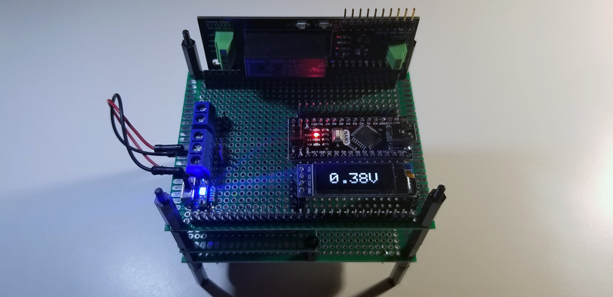
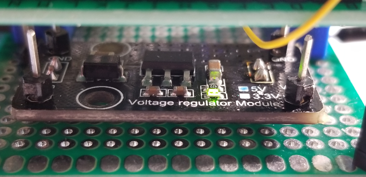
The module is a stacked arrangement of PCBs to allow for the separation of system types by function. The lowest tier hosts two 18650 batteries with a daughterboard with mounted voltage regulators. The batteries attach to the inputs of these regulators as they, in turn, supply the stable voltage supply for the top-tier PCB. The top tier PCB is where the primary functions are for added attachments and interfaces concerning development supported by this system.


With reserved space and pins for added development, two separate terminal blocks are assigned to 5VDC, 3.3VDC, and a completely isolated variable voltage port for higher-current and more sensitive applications. The display is physically reversible and detachable for reuse elsewhere. As the microslot module is socketed for plug-and-go purposes. New projects that become developed in microslot format are rendered compatible by fit and function in this way.

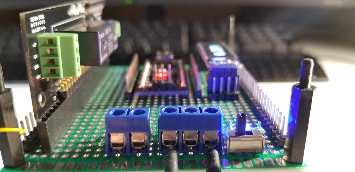
The sockets, terminal blocks, pin headers, and PCB grid provide redundant and variable connectivity options required for suitable flexibility. On the underside of this PCB are the hardwired jumper wires secured and soldered in place.

One regular module for 5V and the other for 3.3V bucks the supply voltage down to the required minimum voltage to the top tier just above it. These are permanently wired to the batteries below.

The two batteries underneath the regulator modules are wired in series to deliver a maximum of 8.4VDC (fully charged). They are easily removable for recharge, and the jumper shunt block is detachable to remove power from the entire system.


Temperature Monitor & Control with a DHT22 Sensor

With a DHT22 (AM2302) temperature and humidity sensor, an Arduino Nano is programmed to activate a relay that in turn permits a fan that provides cooling to a designated system, or target. The relay is set up in a normally open configuration and closes the fan’s contact path to a 5VDC supply when the Arduino Nano asserts its active state. Through a 2N2222 NPN transistor, the relay is given enough signal strength from the Nano GPIO to close and run the fan. The relay’s supply does not operate from USB power, but instead, the entire system runs from its own supply with sufficient current.

While programming the Nano, it is necessary to turn off or disconnect the primary supply to assure no adverse stresses are upon the system. Once the Nano is programmed, in this configuration, the USB plug must be disconnected to operate the primary supply for all other components (relay, fan, transistor, and sensor).

The DHT22 sensor outperforms the DHT11 sensor. Here are the differences:

  • Temperature Range
    • DHT11: -20 to 60℃
    • DHT22: -40 to 80℃
  • Temperature Accuracy
    • DHT11: ±2%
    • DHT22: ±0.5%
  • Humidity Range
    • DHT11: 5 to 95% RH
    • DHT22: 0 to 100% RH
  • Humidity Accuracy
    • DHT11: ±5%
    • DHT22: ±2%
  • Cost
    • DHT11: ~ $6.00
    • DHT22: ~ $10.00

The DHT22 has much lower power consumption, and with a signal transmission distance of more than 20 meters. The sensor operates with a faster measurement response with less interference susceptibility.

Humidity sensor of 0 to 99.9 %RH with ±2% accuracy while the temperature sensor ranges from -40 to 80℃ with ±0.5℃ accuracy.

The relay selected in this project is overkill in terms of its current capacity, but it was readily available since it has a 5VDC input operating voltage. Moreover, the Normally Closed connection isn’t used either. While this relay is a universal relay, there are many available with a lower and much more suitable rating (and cost) for this type of project.

Project Schematic:

The system makes use of the SSD1306 128×64 OLED display to provide a way to monitor the DHT22 sensor’s temperature and humidity readings. Coded into the Nano is a relay and fan trigger activation point as selected. When the DHT22 sensor reads above that temperature level, the fan runs at full speed and remains that way until the temperature again decreases below the set point. If the ambient temperature present at the sensor should again rise above that trigger point, the Nano asserts an active high state and begins the fan’s operating cycle again.

Project Review:

This is the demonstration to verify operation of the OLED display and the fan via the relay as the code set point is chosen at 78-degrees Fahrenheit. When the temperature drops below that point, the fan is disconnected from its 5VDC supply via the relay.


Code Example:

#include “DHT.h”
#include “U8glib.h”
U8GLIB_SSD1306_128X64 u8g (U8G_I2C_OPT_NONE|U8G_I2C_OPT_DEV_0);
#define DHTPIN A0 // Digital pin connected to the DHT sensor

// Uncomment whatever type you’re using
//#define DHTTYPE DHT11 // DHT 11
#define DHTTYPE DHT22 // DHT 22

char str[10];
int relay=5;

DHT dht(DHTPIN, DHTTYPE);

void setup() {
Serial.begin(9600);
Serial.println(F(“Hello James…”));

dht.begin();
u8g.firstPage();
pinMode(relay,OUTPUT);
}

void loop() {
// Wait a few seconds between measurements.
delay(3000);

// Reading temperature or humidity takes about 250 milliseconds
float h = dht.readHumidity();
// Read temperature as Celsius (the default)
//float t = dht.readTemperature()

// Read temperature as Fahrenheit
float t = dht.readTemperature()*1.8+32;

// Check if any reads failed and exit early (to try again).
if (isnan(h) || isnan(t) ) {
Serial.println(F(“Failed to read from DHT sensor.”));
return;
}

Serial.print(t);
Serial.print(“,”);
Serial.println(h);

u8g.firstPage();
do {
u8g.setFont(u8g_font_helvB08);
u8g.drawStr( 0, 15, “[ INSERT TITLE HERE ]”);

u8g.drawStr( 0, 30, “Humidity:”);
u8g.drawStr( 80, 30, dtostrf(h, 5, 2, str));
u8g.drawStr( 110, 30, “%”);

u8g.drawStr( 0, 50, “Temperature:”);
u8g.drawStr( 80, 50, dtostrf(t, 5, 2, str));
u8g.drawStr( 110, 50, “\260F”);
// u8g.drawStr( 110, 50, “\260C”);

if (t>78){
delay(25);
digitalWrite(relay,HIGH);
delay(100);
}
else

if (t<78){
delay(25);
digitalWrite(relay,LOW);
delay(100);
}

}

while( u8g.nextPage() );

}


IMU Acceleration, Gyro, & Magnetometer Calibration

In an effort to produce reliable quantitative angles of tilt and roll of the IMU module, it is necessary to calibrate all 9-axis vectors. Acceleration, gyroscope, and magnetometer are together calibrated together as a single system where reliable calculation and measurement of tilt and roll functions become achievable. In this post, an explanation of how the calibration is done to include visual verification leads to the successful application of tilt and roll measurement as demonstrated. To get an accurate approximation of tilt and roll measurements, calibration of all vectors is necessary. Effectively, this project provides a way to obtain tilt in two different directions using the BNO055 IMU module.

Screen Capture 1 – Calibration data readings that correspond to visual plotting of each combined level to 3,3,3,3. See legend in image that indicates varying levels before stability at achieved calibration.

All four calibration categories must register in the data acquisition stream as 3,3,3,3. Three-axis together as three for each category to include the system which is the combined fused total of the three. When first running the IMU module, or after reset, the data readings will appear at 0 until all four settles into position as 3. To get each to settle (accel, gyro, mag, and sys), it is necessary to physically rotate the IMU module. Move the IMU around in a figure-8 motion and watch for the data readings to rise from 0 to 3.


Sometimes the numbers among all four columns will drop below three, but eventually, they will all four level-out at 3. At times a single column number will not get to three and can appear stubborn. So it is important to hold the IMU in 45-degree roll, tilt, and yaw increments for a few seconds each. That is usually the most effective approach to get all four vectors to align at 3,3,3,3. It is always important to keep the IMU unit away from sources of magnetism, or motors, or sources of EMI that could adversely affect calibration, or an ability to achieve calibration. Keep the IMU away from sources of EMI during calibration while watching for acc, gyro, mag, and sys levels visually plotted and quantitatively acquired in the data readings (see Text View tab).

When all four vector categories are in alignment, it then becomes possible to run tilt and roll tests to obtain reliable confidence in tilt and toll angles of measurement. Notice that the calibration legend is set by category within the Plot tab. Simply double click the Channel name to rename it to a label that is suitable. It is also necessary to set the Auto Scale Y-Axis to a readable number between 0 and 4. That way it is easier to see the variability in calibration by visual recognition. Otherwise, you rely solely on the 3,3,3,3, quantitative measures within the Text View tab as depicted in Screen Capture 1 above.

Screen Capture 2 – Enable calibration channels and set Y Axis Scale for readability of data acquisition.

To monitor tilt and roll it will be necessary to deselect the acceleration, gyro, magnetometer, and system channels to disable the plot and legend. You may want to do this as more serial.print lines in code to display tilt and roll angles will plot separately as additional channels.

Screen Capture 3 – Deselect calibration channels and reset the Y-axis scale for angular data readings. Setting -90 to 90 degrees is better, but for a full range example -180 to 180 is demonstrated here to indicate wide, but accurate variability for the best approximation.

Once calibration is set and the plot graph is ready to display the angular channels (theta and phi), you can physically tilt and roll the IMU module to get positive and negative angles of movement and position. The calculated and plotted serial data that represents rotation along the y-axis is the name theta in this example. It represents a physical tilt action from up (positive) to down (negative) angles of movement. Conversely, the roll motion is physical rotation along the x-axis, so named phi in this example. Physical rotation along the x-axis right (positive) and left (negative) also get plotted and acquired within the data readings within the Text View tab.

Screen Capture 4 – Tilt and roll measurements (+/- degrees of rotation) of both theta and phi with a fully calibrated IMU module.

As written about before, acceleration, gyro, and magnetometer, as separate categories, each has 3-axis degrees of freedom. Where all three together produce a total of 9-degrees of freedom. So, with each category, a unity of 3 for each gives us confidence that they are all together, yet separately, calibrated.

Project Review:

A physical demonstration is captured here both visually and quantitatively. As roll and tilt movement is applied to the IMU module, corresponding positive and negative angles of change become plotted and logged for quantitative analysis.


Tilt & Roll Calculations:

Code Example:

#include <Wire.h>
#include <Adafruit_Sensor.h>
#include <Adafruit_BNO055.h>
#include <utility/imumaths.h> //Within the Adafruit Unified Library
#include <math.h> //Permits inverse tangent function below

float theta;
float phi;

#define BNO055_SAMPLERate_DELAY_MS (100)

/* The myIMU object is self-declared. It can be named any identifier.*/
Adafruit_BNO055 myIMU = Adafruit_BNO055();

void setup()
{
Serial.begin(115200);
myIMU.begin();
delay(1000);

/* The in8_t is a very compact data type:*/
int8_t temp=myIMU.getTemp();

/* Instruction to use the onboard BNO055 VCXO, not on the MPU chip itself:*/
myIMU.setExtCrystalUse(true);
}

void loop()
{

uint8_t system=0, gyro=0, accel=0, mg=0; /*Byte sized variable data type */
myIMU.getCalibration(&system, &gyro, &accel, &mg);
imu::Vector<3> acc =myIMU.getVector(Adafruit_BNO055::VECTOR_ACCELEROMETER);

/*A calculated approximation of tilt (inverse tangent (ax/9.8) divided by (az/9.8)).
The 9.8 denominator in each term is to normalize the vector to 1-g for each variable.
Then dividing by 2 and 3.14 (pi) converts the measurement units to degrees.*/

theta=-atan2(acc.x()/9.8,acc.z()/9.8)/2/3.141592654*360;
phi=-atan2(acc.y()/9.8,acc.z()/9.8)/2/3.141592654*360;


Serial.print(acc.x()/9.8);
Serial.print(“,”);
Serial.print(acc.y()/9.8);
Serial.print(“,”);
Serial.print(acc.z()/9.8);
Serial.print(“,”);
Serial.print(accel);
Serial.print(“,”);
Serial.print(gyro);
Serial.print(“,”);
Serial.print(mg);
Serial.print(“,”);
Serial.print(system);
Serial.print(“,”);
Serial.print(theta);
Serial.print(“,”);
Serial.println(phi);

/* Insert delay to assure you’re not going faster than what the sensor can handle. */
delay(BNO055_SAMPLERATE_DELAY_MS);
}


IMU Data Serial Plotter Setup and Configuration

Similar to the serial plotter on the Arduino Sketch IDE, there is a useful real-time serial plotter application at the Hackaday site. It is free and it offers configuration options that add to the utility of data tracking, measurement, and analysis. The application provides for scroll, zoom, cursor, channel selections, and color options that ease how visually parsed data is presented and managed. There is a range of capabilities with the utility that makes it a better way to go over the Sketch IDE data plotter.

Example data acquisition from plotted data points over time.

While the link provided gives a way to download and install the latest data plotter version, this post makes use of the following file:

Once the utility is installed and running, there are configuration options I use to monitor the IMU serial data streams. Specifically, it is necessary to select the available COM port connected to the USB port on the Arduino host of the IMU module. Once that is done, the Baud Rate selected within the application’s Port tab must match the baud rate declared in the void setup() segment of your Arduino code. In this example, my declaration is Serial.begin(115200), so the baud rate selection must be 115200). The standard serial handshaking configurations apply as 8-bit, 1 stop bit, no parity, and no flow control.

It is important that the Arduino Sketch serial plotter application isn’t running as it will present a conflict with this utility.

Screen Capture 1 – Port selection and baud rate.

Next is formatting the data according to how the vector data acquisition code is written as an ASCII data type and for proper delimiting. Since the comma it used for data capture, that option is selected.

Screen Capture 2 – Data type and delimiter settings
Screen Capture 3 – Program code that declares the comma.
Screen Capture 4 – Sketch IDE Serial Monitor that streams acquired data with comma separation / delimiting.

While the three acceleration vectors x, y, z automatically populated according to the number of channels in screen capture two (2) above. To add more channels (vectors), simply increase the quantity from the data format tab. The buffer size setting corresponds to the vector data held in memory and gets displayed along the x-axis in the plotter graph. Setting the plot width to a narrow data window increases the plotted data acquisition rate from right to left. The scale axis settings simply correspond to the amplitude of inflections observed in the data.

Screen Capture 5 – Data plotter configuration. Double-click each channel field within the Plot tab to name the data as desired for legend placement and identification.

The other four tabs have less relevance in the set up here, but they are useful to record and monitor data as an output to acquired data. To further explore settings for visual quality and precision, experiment with the menu options to get your desired layout and format.

Screen Capture 6 – Layout and graphical format options for visual quality.
Screen Capture 7 – Zoom window by cursor selection to expand and view further into data points. Right click within the pane to reset full view.
Screen Capture 8 – Zoomed in view of acquired data segment.

Project Review:


BNO055 IMU 9-Axis DOF Acceleration Analysis

In an effort to further delve into the inner workings of the BNO055 accelerometer and its functions, the serial plotter was applied to the project. To better understand how the produced data is rendered over the I2C SDA/SCL connection to the Nano, the data is translated by the plotter into a visual char as presented below. The gyro and magneto functions of the IMU are not included in this review to get a better depth of understanding around the module’s capabilities.

The amount of capacitive charge capacity within a capacitor. The permittivity of an insulator (ε) describes the insulator’s resistance to the creation of an electric field and is equal to 8.85×10⁻¹² Farads per meter for an air-gap capacitor.

The three-axis of acceleration is plotted over time as a function of latitude movement (x-axis), longitude movement (y-axis), and vertical movement (z-axis). As the IMU module is moved and oriented to different positions, the sensor interprets that activity by measurement of differences in charge. Specifically, internally charged surfaces are separated by differences in area and distance to vary a combined capacitive charge. That change in charge, as measured, corresponds to the difference in acceleration since internal plate movement varies in all three directions.

In the photo here, imagine that a lower plate is moving up and down, back and forth through its comb structure. The surface area for each direction of movement brings about a difference in capacitive charge where that becomes interpreted as acceleration. The substrate below the comb structure consists of a surface area that corresponds to the z-axis charge that is tracked for changes in vertical acceleration. The lattice framed structure is suspended by springs to assure continuous and precise movement in any direction within defined limits.

It is again useful to recognize that the amount of charge present within the capacitor, or capacitive body, is determined by the surface area and distance between two charged plates. Reduce the surface area between the two plates, and the total capacitive charge is reduced. Increase the distance between the two plates and the capacitive charge is reduced. This simplified explanation does not take into account any dielectric properties that exist among different types of capacitors.

Red: X-axis latitude acceleration. Blue: Y-axis longitude acceleration. Green: Z-axis vertical. Notice that the green plot is tracking at
9.8m/s2 since that is the acceleration of gravity present at the IMU module. The -9.8m/s2 reading is with the IMU inverted with the internal
micro-electro-mechanical (MEM) structure pulled down by gravity.

Project Schematic:

The same basic connections are in place as before in the prior set up project. The key I2C communication connections between the modules remain in place to transfer clock and data for integration and processing. Both modules share the same ground and 5V VCC.

Project Review:

As demonstrated in this video, the IMU module’s data plot extends across time as the acceleration tests are carried out. As the IMU module is moved to different positions and orientations, observe the corresponding changes in plotted graphical data.


Code Example:

#include <Wire.h>
#include <Adafruit_Sensor.h>
#include <Adafruit_BNO055.h>

/* Within the Adafruit Unified Library*/
#include <utility/imumaths.h>

#define BNO055_SAMPLERATE_DELAY_MS (100)

/* The myIMU object is self-declared. It can be named any identifier.*/
Adafruit_BNO055 myIMU = Adafruit_BNO055();

void setup()
{
Serial.begin(115200);
myIMU.begin();
delay(1000);

/* The in8_t is a very compact data type:*/
int8_t temp=myIMU.getTemp();

/* Instruction to use the onboard BNO055 VCXO, not on the MPU chip itself:*/
myIMU.setExtCrystalUse(true);
}

void loop()
{
imu::Vector<3> acc =myIMU.getVector(Adafruit_BNO055::VECTOR_ACCELEROMETER);
Serial.print(acc.x());
Serial.print(“,”);
Serial.print(acc.y());
Serial.print(“,”);
Serial.println(acc.z());

/* Insert delay to assure you’re not going faster than what the sensor can handle. */
delay(BNO055_SAMPLERATE_DELAY_MS);
}


BNO055 IMU 9-Axis DOF Hardware & Software Setup

Once initial hardware is in place, it is necessary to gather the libraries to run the software and get connectivity and begin gathering the Arduino unit and the BNO055 IMU Fusion module data. In this setup, various libraries are needed to run the code as it becomes developed in this post and further along among projects.

Project Schematic:

The physical build of the IMU assembly is very simple. Wiring between the IMU module and the Arduino Nano is as illustrated in the schematic below.

BNO055 Module:

The pins on the BNO055 are laterally interspersed by function. Namely, Power, I2C, and Utility. With VIN, 3VO, and Ground as the power input pins, the SDA (serial-data) and SCL (serial clock) are the I2C pins, and finally a mix of addressing, interrupt and mode pins (RST, INT, ADR, & PS0/PS1).

BNO055 Pinout:

PinNameDescription
1VIN3.3-5.0V power supply input
23VO3.3V output from the onboard linear voltage regulator, you can draw up to about 50mA.
3GNDThe common/GND pin for power and logic.
4SDAI2C data pin, connect to your microcontroller’s I2C data line. This pin can be used with 3V or 5V logic, and there’s a 10K pullup on this pin.
5SCLI2C data pin, connect to your microcontroller’s I2C data line. This pin can be used with 3V or 5V logic, and there’s a 10K pullup on this pin.
6RSTHardware reset pin. Set this pin low then high to cause a reset on the sensor. This pin is 5V safe.
7ADRSet this pin high to change the default I2C address for the BNO055 if you need to connect two ICs on the same I2C bus. The default address is 0x28. If this pin is connected to 3V, the address will be 0x29.
8INTThe HW interrupt output pin, which can be configured to generate an interrupt signal when certain events occur like movement detected by the accelerometer, etc. (not currently supported in the Adafruit library, but the chip and HW are capable of generating this signal). The voltage level out is 3V.
9PS1This pin can be used to change the mode of the device (it can also do HID-I2C and UART) and also is provided in case Bosch provides a firmware update at some point for the ARM Cortex M0 MCU inside the sensor. Should normally be left unconnected.
10PS0This pin can be used to change the mode of the device (it can also do HID-I2C and UART) and also is provided in case Bosch provides a firmware update at some point for the ARM Cortex M0 MCU inside the sensor. Should normally be left unconnected.

Project Review:

The physical movement of the IMU along the various degrees of freedom (DOF), produces vector data as demonstrated in this video. A before and after comparison of the data by a change of position indicates changes in the acceleration and gyroscope to validate positive and negative orientation.


Arduino IDE:

Arduino Libraries:

Arduino Serial Monitor:

Once a suitable serial COM port is selected from the tools menu, access to the Serial monitor is made available to call for its use in the setup code of the program (under void setup()) function as Serial.begin([baudrate]).

Select Suitable COM Port

Select Serial Monitor

View Serial Monitor for Vector Data

Code Example:

#include <Wire.h>
#include <Adafruit_Sensor.h>
#include <Adafruit_BNO055.h>
#include <utility/imumaths.h> //Within the Adafruit Unified Library

//The myIMU object is self-declared. It can be named any identifier.
Adafruit_BNO055 myIMU = Adafruit_BNO055();

void setup()
{
Serial.begin(9600);
myIMU.begin();
delay(1000);

//The in8_t is a very compact data type:
int8_t temp=myIMU.getTemp();

//Instruction to use the onboard BNO055 VCXO, not on the MPU chip itself:
myIMU.setExtCrystalUse(true);
}

void loop()
{
/*Go out to the IMU and return vector data with 3-components into
acc (accelerometer) named variable and store it into the created
object myIMU with the accelerometer parameter (since there are
three-axis x,y,&z). */

imu::Vector<3> acc =myIMU.getVector(Adafruit_BNO055::VECTOR_ACCELEROMETER);

/*Go out to the IMU and return vector data with 3-components into
gyro (gyroscope) named variable and store it into the created
object myIMU with the gyroscope parameter (since there are
three-axis x,y,&z). */

imu::Vector<3> gyro =myIMU.getVector(Adafruit_BNO055::VECTOR_GYROSCOPE);

/*Go out to the IMU and return vector data with 3-components into mag (magnetometer) named variable and store it into the created object myIMU with the magnetometer parameter (since there are three-axis x,y,&z). */

imu::Vector<3> mag =myIMU.getVector(Adafruit_BNO055::VECTOR_MAGNETOMETER);

Serial.print(“Acceleration X-Vector: “);
Serial.println(acc.x());
Serial.print(“Acceleration Y-Vector: “);
Serial.println(acc.y());
Serial.print(“Acceleration Z-Vector: “);
Serial.println(acc.z());
Serial.println(” “);
Serial.print(“Gyroscope X-Vector: “);
Serial.println(gyro.x());
Serial.print(“Gyroscope Y-Vector: “);
Serial.println(gyro.y());
Serial.print(“Gyroscope Z-Vector: “);
Serial.println(gyro.z());
Serial.println(” “);
Serial.print(“Magnetometer X-Vector: “);
Serial.println(mag.x());
Serial.print(“Magnetometer Y-Vector: “);
Serial.println(mag.y());
Serial.print(“Magnetometer Z-Vector: “);
Serial.println(mag.z());
Serial.println(” “);

/* Insert delay to assure you’re not going faster than what the sensor can handle. */
delay(BNO055_SAMPLERATE_DELAY_MS);
}


LED Matrix Display with Single Digit Messaging

The LED Matrix display in this project can be more versatile than other typical LED indicators. Standard LEDs and 7-segment LEDs have their unique or dedicated purpose for readout or illumination to indicate activity or an event, but this matrix display offers variable messaging capabilities. From within the code driving this display, either visual characters or images are display in a sequential fashion to convey messages.


Set up is easy with only three terminations between both the display and the Arduino Nano/Uno. Aside from VCC and ground, CLK (clock), CS (chip-select), and DIN (data-input) are terminated to GPIO pins D12 through D10 respectively. As illustrated in the schematic below the connections are defined for clarity.

Project Schematic:

Project Review:

Running the project is straight-forward with each dot of light representing a single LED element. When combined together, or as a sequence, the display acts as pixels do on a monitory to form characters and images. Only on this display with a higher intensity of light.


Code Example:

#include <LedControl.h>

/* Need a LedControl to work with.
pin 12 is connected to the DIN (data input)
pin 11 is connected to CS
pin 10 is connected to the CLK */

LedControl lc=LedControl(12,10,11,1);

/* Always wait a bit between updates of the display */

unsigned long delaytime1=500;
unsigned long delaytime2=5;

void setup()
{
/* The MAX72XX is in power-saving mode on startup,
it is necessary to wake up the display */
lc.shutdown(0,false);

/* Set the brightness to a medium values */
lc.setIntensity(0,8);

/* Clear the display */
lc.clearDisplay(0);
}

/* This method will display the characters for the word “Arduino” one after the other on the matrix (you need at least 5×7 LEDs to see the whole chars). */

void writeArduinoOnMatrix()
{
/* here is the data for the characters */
byte a[5]={B01111110,B10001000,B10001000,B10001000,B01111110};
byte r[5]={B00010000,B00100000,B00100000,B00010000,B00111110};
byte d[5]={B11111110,B00010010,B00100010,B00100010,B00011100};
byte u[5]={B00111110,B00000100,B00000010,B00000010,B00111100};
byte i[5]={B00000000,B00000010,B10111110,B00100010,B00000000};
byte n[5]={B00011110,B00100000,B00100000,B00010000,B00111110};
byte o[5]={B00011100,B00100010,B00100010,B00100010,B00011100};

/* now display them one by one with a small delay */
lc.setRow(0,0,a[0]);
lc.setRow(0,1,a[1]);
lc.setRow(0,2,a[2]);
lc.setRow(0,3,a[3]);
lc.setRow(0,4,a[4]);
delay(delaytime1);
lc.setRow(0,0,r[0]);
lc.setRow(0,1,r[1]);
lc.setRow(0,2,r[2]);
lc.setRow(0,3,r[3]);
lc.setRow(0,4,r[4]);
delay(delaytime1);
lc.setRow(0,0,d[0]);
lc.setRow(0,1,d[1]);
lc.setRow(0,2,d[2]);
lc.setRow(0,3,d[3]);
lc.setRow(0,4,d[4]);
delay(delaytime1);
lc.setRow(0,0,u[0]);
lc.setRow(0,1,u[1]);
lc.setRow(0,2,u[2]);
lc.setRow(0,3,u[3]);
lc.setRow(0,4,u[4]);
delay(delaytime1);
lc.setRow(0,0,i[0]);
lc.setRow(0,1,i[1]);
lc.setRow(0,2,i[2]);
lc.setRow(0,3,i[3]);
lc.setRow(0,4,i[4]);
delay(delaytime1);
lc.setRow(0,0,n[0]);
lc.setRow(0,1,n[1]);
lc.setRow(0,2,n[2]);
lc.setRow(0,3,n[3]);
lc.setRow(0,4,n[4]);
delay(delaytime1);
lc.setRow(0,0,o[0]);
lc.setRow(0,1,o[1]);
lc.setRow(0,2,o[2]);
lc.setRow(0,3,o[3]);
lc.setRow(0,4,o[4]);
delay(delaytime1);
lc.setRow(0,0,0);
lc.setRow(0,1,0);
lc.setRow(0,2,0);
lc.setRow(0,3,0);
lc.setRow(0,4,0);
delay(delaytime1);
}

/* This function lights up some LEDs in a row.
The pattern will be repeated on every row.
The pattern will blink along with the row-number.
row number 4 (index==3) will blink 4 times etc. */

void rows() {
for(int row=0;row<8;row++) {
delay(delaytime2);
lc.setRow(0,row,B10100000);
delay(delaytime2);
lc.setRow(0,row,(byte)0);
for(int i=0;i<row;i++) {
delay(delaytime2);
lc.setRow(0,row,B10100000);
delay(delaytime2);
lc.setRow(0,row,(byte)0);
}
}
}

/*This function lights up some LEDs in a column.
The pattern will be repeated in every column.
The pattern will blink along with the column-number.
column number 4 (index==3) will blink 4 times etc. */

void columns() {
for(int col=0;col<8;col++) {
delay(delaytime2);
lc.setColumn(0,col,B10100000);
delay(delaytime2);
lc.setColumn(0,col,(byte)0);
for(int i=0;i<col;i++) {
delay(delaytime2);
lc.setColumn(0,col,B10100000);
delay(delaytime2);
lc.setColumn(0,col,(byte)0);
}
}
}

/* This function will light up every Led on the matrix.
The led will blink along with the row-number.
row number 4 (index==3) will blink 4 times etc. */

void single() {
for(int row=0;row<8;row++) {
for(int col=0;col<8;col++) {
delay(delaytime2);
lc.setLed(0,row,col,true);
delay(delaytime2);
for(int i=0;i<col;i++) {
lc.setLed(0,row,col,false);
delay(delaytime2);
lc.setLed(0,row,col,true);
delay(delaytime2);
}
}
}
}

void loop() {
writeArduinoOnMatrix();
rows();
columns();
single();
}


Motion Detector with Passive Infrared (PIR) Sensor

This project involves a motion detector that “observes” its immediate environment to inform the Arduino that an active state change is present. The Arduino in turn processes that state change for code-driven events to make the motion detector a useful device that monitor’s the physical movement of objects in its immediate environment.

The HC-SR501 passive infrared sensor in this project is not an obvious type of sensor to understand in a traditional sense. It consists of active and passive components that facilitate sensitivity and trigger functions that are helpful in its implementation. Two onboard trim pots are adjustment settings that help make the sensor more user friendly. The first concerns the sensor’s distance sensitivity and the second for a time delay after each motion event is triggered.

Further information concerning the sensor with this example is more completely covered in this document.

The sensor dome lens in this image helps to support its 110° conical range of view. From the base of the sensor extending out between 3 to 7 meters, according to its adjusted sensitivity, motion detection is limited within this viewing area.

The Passive Infrared Sensor (PIR) detects motion from within its viewing range by the user settings on the HC-SR501 device itself. Two trim potentiometer adjustments with jumper positions as depicted and explained below set the sensor’s interpretation capabilities as defined.

Upon startup, the PIR device requires about 1-minute to initialize. Since the device will output false detection signals, it is necessary to assure associated readings within interfacing circuit logic takes this condition into account.

The viewing area range, as indicated below, is adjustable with two side-by-side trim pots. The sensitivity trim adjustment on the right of the photo above rotates clockwise or counter-clockwise. Fully clockwise sets the sensor’s viewing range to about 3-meters. Fully counter-clockwise sets the sensor’s viewing range to about 7-meters. Variability between these two settings provide for a distance calibration to support an optimum use-case viewing distance.

During evaluation or experimentation, it is useful to orient the sensors to suitable positions where detection possibilities are assured. The HC-SR501 doesn’t provide for a suitable, or easy mounting solution to a vector or perforated board unless small standoffs are added to each side of the sensor through the PCB mounting holes (about 1.9 – 2.0mm I.D.).

The trim adjustment on the left in the photo above provides for a clockwise and counter-clockwise rotation as well. Fully clockwise increases the delay between detection events to about 5-minutes. Fully counter-clockwise sets the delay to about 3-seconds. This delay occurs after each detection event. It is after each motion detection occurrence that this device signal will go LOW until the set delay is completed. During this delay time, each new detection within the sensor’s viewing range is blocked. Once the delay is completed, any detected motion sets the device output to HIGH. The same delay and detection cycle repeats with these intervals as defined by the sensitivity and viewing range adjustment settings.

The HC-SR501 PIR sensor has three output pins VCC, Output and Ground. It has a DC voltage regulator that accepts 4.5 to 12 volts, so a 5V source is common. The BISS0001 IC is a signal processing chip while diode in the upper left of the photo above is for excess voltage projection. The remaining components are passive resistors and capacitors.

  • Time Delay Adjust: This sets how long the output remains high after detecting motion. Anywhere from about 5 seconds to 5 minutes.
  • Sensitivity Adjust: Sets the detection range of motion from about 3 meters to 7 meters.
  • Trigger Selection Jumper: Set for Single or Repeat trigger events.
  • Ground Pin: Input connection for ground reference.
  • Output Pin: LOW (0V) when no motion is detected and HIGH (3.3V) when motion is detected.
  • VCC Pin: 5VDC to 12VDC input.

The lens cap of the motion detector is easily removable to reveal the PIR sensor mounted to its PCB. The small plastic guideposts are inserted into the PCB to also reveal that the lens cap is detachable. The pinout references for the connector header below are named on the top side of the PCB assembly.

As there are three connection terminals (5V, Ground, and Output), it is also possible to run the sensor freestanding on its own. With 4x AA batteries, a 220 resistor, and an LED, the module operates as a portable yet simple detector for placement just about anywhere practical. For example, a completed assembly in this way can be set in another room where the LED is in viewing distance (or by mirror/camera placement), where it becomes possible to get a primitive notification that someone has entered into that room without you being there.

RT– This is for a thermistor or temperature-sensitive resistor. Adding this allows the HC-SR501 to be used in extreme temperatures, it also increases the accuracy of the detector to some degree. RL– This connection is for a Light Dependent Resistor (LDR) or Photoresistor. By adding this component the HC-SR501 will only operate in darkness, a common application for motion-sensitive lighting systems. The additional components can be soldered directly to the board or extended to remote locations using wires and connectors.

Project Schematic:

The operating voltage of the HC-SR501 is between 5VDC and 12VDC, but in this example using the Arduino Nano it is supply with the same 5VDC source. The LED (D1) is the signal light to indicate when the senor has detected motion.

Project Review:

This motion detection experiment checks for illumination activity as movement is placed before the sensor and just out of range. Additional movement tests are performed while the sensor is in the block state for the duration set by the timing adjustment at the trim potentiometer on the module. The reset of the sensor (and LED) activity is made evident with the jumper setting as described above.


Code Example 1:

This code simply illuminates the LED when motion is detected.

int ledPin = 4; // LED on pin 4 of Arduino
int pirPin = 7; // HC-S501 sensor input to Arduino

int pirValue; // Variable to read PIR Value

void setup()
{
pinMode(ledPin, OUTPUT);
pinMode(pirPin, INPUT);
digitalWrite(ledPin, LOW);
}

void loop()
{
pirValue = digitalRead(pirPin);
digitalWrite(ledPin, pirValue);
}

Code Example 2:

This code illuminates the LED and sends a message to the serial monitor when motion is detected.

int ledPin = 4; // choose the pin for the LED
int inputPin = 7; // choose the input pin (for PIR sensor)
int pirState = LOW; // we start, assuming no motion detected
int val = 0; // variable for reading the pin status

void setup()
{
pinMode(ledPin, OUTPUT); // declare LED as output
pinMode(inputPin, INPUT); // declare sensor as input
Serial.begin(9600);
}

void loop()
{
val = digitalRead(inputPin); // read input value
if (val == HIGH) // check if the input is HIGH
{
digitalWrite(ledPin, HIGH); // turn LED ON

if (pirState == LOW)
{
Serial.println(“Motion Detected!”); // print on output change
pirState = HIGH;
}
}
else
{
digitalWrite(ledPin, LOW); // turn LED OFF

if (pirState == HIGH)
{
Serial.println(“Motion Detected!”); // print on output change
pirState = LOW;
}
}
}


Binary Counter, Logic & Circular Shift Register

The 74HC595 is a CMOS logic device that functions as an 8-bit Serial-Input / Serial or Parallel-Output shift register with latched 3-State Outputs. The shift register accepts serial data and provides a serial output. The shift register also provides parallel data to the 8–bit latch. The shift register and latch have independent clock inputs. This device also has an asynchronous reset for the shift register. It is especially useful as it directly interfaces with the SPI serial data port on CMOS MPUs and MCUs.

This project demonstrates the typical practical use of the shift register by counting up in binary from 0 to 255. It shifts the presence of serial data from right to left and left to right as that data is clocked through the register from an Arduino Nano. The Nano provides the data, the clock, and latch control to present output data to an LED array.

As inputs are cycled through the register, binary state changes are visually represented at the LED array. Each LED from left to right is a single bit from 0 to 7. Left most LED is the most significant bit (MSB) and the right most LED is the least significant bit (LSB). The two LEDs at the right end of the array are inactive in this project.

The datasheet of the 74HC595 provides added details concerning operating descriptions, limits, timing waveforms, testing conditions, and packaging. The purpose of the device centers around the conversion of serial input data to serial or parallel outputs through its internal shift register. Most typically, as serial data is applied to the register’s input, the data becomes transposed to parallel outputs across 8 separate pins. Outputs present at those pins are held as a latch until delivery is permitted by a control pin to deliver serial data when desired as a matter of timing or synchronization.

Pin Descriptions
INPUTS
A (Pin 14)
Serial Data Input. The data on this pin is shifted into the
8–bit serial shift register.
CONTROL INPUTS
Shift Clock (Pin 11)

Shift Register Clock Input. A low– to–high transition on
this input causes the data at the
Reset (Pin 10)
Active–low, Asynchronous, Shift Register Reset Input. A
low on this pin resets the shift register portion of this device
only. The 8–bit latch is not affected.
Latch Clock (Pin 12)
Storage Latch Clock Input. A low–to–high transition on
this input latches the shift register data.
Output Enable (Pin 13)
Active–low Output Enable. A low on this input allows the
data from the latches to be presented at the outputs. A high
on this input forces the outputs (QA–QH) into the
high–impedance state. The serial output is not affected by
this control unit.
OUTPUTS
QA – QH (Pins 15, 1, 2, 3, 4, 5, 6, 7)

Noninverted, 3–state, latch outputs.
SQH (Pin 9)
Noninverted, Serial Data Output. This is the output of the
eighth stage of the 8–bit shift register. This output does not
have three–state capability.

Project Schematic:

The system components consist of an Arduino Nano, a 74HC595 8-bit shift register, a 100-ohm resistor pack, and an LED array. Together these components are assembled to support the code necessary to deliver computer or user data to a collection of outputs (QA through QH). All 8-bits of data are shifted through the device from the Arduino (pin 9) to the shift register control (pin 11). The serial data received at pin 14 of the register becomes internally transposed and placed to outputs QA through QH as the data is latch clocked on its state transitions to the outputs via the R-clock control pin at pin 12.

74HC595 Logic Diagram:

Data and control functions indicate the serial input to parallel output states made possible through grouped flip-flops. State propagation is triggered among all flip flops through latch clock edge transitions as illustrated at each flip flop in the diagram.

Flip-flop groups that shifts and holds data to sequentially transition all states to separate outputs. Each flip-flop physically represents a single register position.

Project Review:


Code Example:

int latchPin=11;
int clockPin=9;
int dataPin=12;
int dt=100;
byte Bytes=0b11111110; //circular shift left with 1 LED Off
//byte Bytes=0b00000001; //circular shift left with 1 LED On

void setup()
{
Serial.begin(9600);
pinMode(latchPin,OUTPUT);
pinMode(dataPin,OUTPUT);
pinMode(clockPin,OUTPUT);
}

void loop()
{
digitalWrite(latchPin,LOW);
shiftOut(dataPin,clockPin,LSBFIRST,Bytes);
digitalWrite(latchPin,HIGH);
delay(dt);
Serial.println(Bytes);
Bytes=Bytes/128+Bytes2; // circular shift left
//Bytes=Bytes128+Bytes/2; // circular shift right
}


Smoke Detector with Alarm and LED Indicators

While the MQ-2 gas sensor is one among a range of gas sensor types, it is roughly suitable for coarse experimentation for substances other than smoke. This sensor is sensitive to smoke and Liquid Petroleum Gas (LPG), Butane, Propane, Methane, Alcohol, and Hydrogen, but this project is set up for smoke detection to further explore its functionality, capabilities, and limitations.

The project includes a sensor to detect smoke as an input source that senses the presence of flammable gases or the origination of smoke and smoke itself in its immediate environment. The circuit is assembled to also include a buzzer alarm and two LEDs to indicate status (red for alarm and green for normal). While the sensor sits in its free space, it detects normal levels of air as a comparison to any gases or smoke that might be mixed in. That normal level is a threshold set with a sensitivity setting on the sensor itself (a small trim potentiometer).

The alarm and status LED changes are triggered from a threshold set within code according to the sensitivity setting trimmed as a configuration at the sensor. The range of high or low sensitivity is limited to the specifications of the sensor.

Project Schematic:

Assembly of this project is a simple effort to connect all relevant components. Three 330-ohm resistors, 1 active buzzer, 1 green LED, 1 red LED, 1 MQ-2 gas sensor, and an Arduino Nano with a USB-Mini connection to a computer for programming support. The Arduino Nano also provides power for the circuit as a whole while it is in operation.

Smoke Detector Circuit using the MQ-2 Gas Sensor.

Project Review:

An incense stick was safely lit to produce the smoke necessary to run this test. As smoke is presented to the sensor from the incense stick, the detector sets off the alarm and illuminates the LED as expected. When the smoke is removed from the sensor’s proximity, the system automatically returns to normal as expected.


Code Example:

While this code is for generic evaluation use, it is further expected to calibrate the detector’s sensor by first setting it into free air within its environment and establish a low/high condition with respect to ambient humidity and temperature. As a range, the threshold level set within code and trimmed on the sensor should take into account normal air conditions excluding the presence of smoke. The calibration level within a +/- range is not set within this project, but it is important to take these conditions into account for more precise applications. This project is simply for rough experimentation with a default threshold value trimmed with a wide latitude for variability in air quality or conditions.

//For MQ-2 Gas Sensor

int redLed = 12;
int greenLed = 11;
int buzzer = 10;
int smoke = A5;

/* Set threshold value then trim sensor value (read from Serial Monitor) at a % below to account for the range of variation in humidity and temperature. */

int sensorThreshold = 400;

void setup()
{
pinMode(redLed, OUTPUT);
pinMode(greenLed, OUTPUT);
pinMode(buzzer, OUTPUT);
pinMode(smoke, INPUT);
Serial.begin(9600);
}

void loop()
{
int analogSensor = analogRead(smoke);

Serial.print(“Sensor Reading: “);
Serial.println(analogSensor);
// Checks if it has reached the threshold value
if (analogSensor > sensorThreshold)
{
digitalWrite(redLed, HIGH);
digitalWrite(greenLed, LOW);
tone(buzzer, 1000, 200);
}
else
{
digitalWrite(redLed, LOW);
digitalWrite(greenLed, HIGH);
noTone(buzzer);
}
delay(100);
}


Flame Detection with Sound Alert & Warning Light

An Arduino Nano is set up in this project to run a flame detection sensor as a small fire alarm system. The system uses a small active buzzer (muted) and an LED to both simulate an alarm condition with the presence of fire in proximity to the flame detector. The Nano was chosen in this project to support any desire for portability or placement into a container that has an internal and temporary battery back up.

The buzzer and LED are visual and audible indicators to simulate an event trigger such as a relay closure to suppress a fire, or shut off a fuel pump. The sensor assembly itself consists of an infrared receiver (IR photodiode), an LM393 op-amp, an SMD power LED, an SMD fire presence LED, a 100k-ohm trim pot, and various resistors for the LED and to compose the op-amp circuit. The trim pot provides and adjustment setting for flame sensitivity at nearby or farther distances.

When the flame sensor detects the presence of fire, its D0 pin produces a logic HIGH output voltage that in turn is read into the Arduino GPIO input pin (pin D4). If there is no flame within proximity of the sensor, the detector returns its D0 output pin to an active LOW state. Where again the Arduino reads that change as an input and interprets the condition for a different event (alarm off, light off, event trigger(s) back to normal).

Project Schematic:

In addition to various jumpers, the project requires a small collection of common and readily available components. Their connections illustrated in this schematic diagram how to connect the various components together using jumper wires. The Arduino unit itself requires its own USB plug to give it and surrounding circuit components power. The same USB connection serves as the programming port to upload the code written to operate the system.

Schematic diagram of Flame Detection circuit.

Project Review:

This short video provides a physical demonstration of how the flame detector operates. As a flame is put in nearby proximity of the sensor, it triggers a computer message, “FIRE ALERT” and it sounds off a buzzer alarm and illuminates a blinking light. The flame is moved shorter and longer distances away from the detector to visibly and audibly recognize the system’s detection threshold.


Arduino IDE:

Code Example:

int buzzer = 8;
int LED = 7;
int flame_sensor = 4;
int flame_detected;

void setup()
{
Serial.begin(9600);
pinMode(buzzer,OUTPUT);
pinMode(LED,OUTPUT);
pinMode(flame_sensor,INPUT);
}
void loop()
{
flame_detected = digitalRead(flame_sensor);
if (flame_detected == 1)
{
Serial.println(“FIRE ALERT!”);
digitalWrite(buzzer, HIGH);
digitalWrite(LED, HIGH);
delay(200);
digitalWrite(LED, LOW);
delay(200);
}
else
{
Serial.println(“Status Normal”);
digitalWrite(buzzer, LOW);
digitalWrite(LED, LOW);
}
delay(1000);
}


Arduino Clone Bootloader Setup & Programming

Arduino modules (in this case an Arduino Nano 3.0) may come from China without the hardware initialized with a suitable bootloader. Necessary for project work and programming, a bootloader configuration is necessary for an Arduino to connect to a local host computer and its Arduino Sketch IDE. To install a bootloader into the clone Arduino, it is necessary to connect it to a known functional Arduino unit (in this example another Nano) and configure the functional Arduino to set up and configure the bootloader code for the target Arduino clone.

Side by side are the source and target Arduino units to set up and configure the bootloader at the target device (the black Arduino Nano).

Once the bootloader set up and programming is successful, the clone Arduino is prepared for standard project work and programming as desired.

A host computer connects to the source Arduino Nano via USB-Mini male to USB-A male. From there, the source Arduino Nano serves as a host for the target Arduino clone. Bootloader code that resides in the source is transferred to the clone with the connections made and the burn utility within the Arduino IDE.

Programming Method

Step 1 | Configure IDE and Load Arduino ISP

  1. Connect functional Arduino to the USB port on your computer. A USB-Mini male to USB-A male cable is necessary to make this connection. No USB connection is made to the clone Arduino.
  2. Open the Arduino IDE software.
  3. Select the correct COM port available from the Arduino menu (Tools > Port > Serial ports). Choose one COM port such as COM1, COM3, COM5, etc.
  4. Select the correct Arduino board from the Boards Manager menu option (Tools > Board: Arduino Nano (in this example).
  5. Open Arduino ISP to functional Arduino connected to the host computer via USB mini (Nano) to USB-A (computer). To open the Arduino ISP file select the correct example file (File > Examples > Arduino ISP). Once selected, the Arduino ISP code should open within the Arduino IDE as a Sketch.
  6. Upload the Arduino ISP code to the functional Arduino (Nano in this case).
  7. Unplug the functional Arduino USB cable and complete the six connections to the clone Arduino as described in step 2 below.

If the Arduino ISP code is needed separately (step 5 above), see the download button/link below.

Step 2 | Connect Arduinos

  1. Connect pin 1 on Arduino clone to D12 of functional Arduino.
  2. Connect pin 2 on Arduino clone to 5V of functional Arduino.
  3. Connect pin 3 on Arduino clone to D13 of functional Arduino.
  4. Connect pin 4 on Arduino clone to D11 of functional Arduino.
  5. Connect pin 5 on Arduino clone to D10 of functional Arduino.
  6. Connect pin 6 on Arduino clone to GND of functional Arduino.

Wiring Schematic

This diagram illustrates how to connect both a functional and clone Arduino together for bootloader programming to the clone. Important: connections D10 – D13 (digital pins 10-13 of the functional Arduino) are the connections to the clone Arduino. For example, do not connect reset or RST of the functional Arduino to the RST of the clone Arduino. Instead, connect D10 of the functional Arduino to pin 5 of the clone Arduino.

Schematic diagram of source and target Arduino units for bootloader upload to a clone Arduino.

Proceed to step 3 below once all connections are made as described in step 2 above, or as illustrated in the wiring schematic above.

Step 3 | Code Load Bootloader

  1. Connect the USB cable to the functional Arduino again for power and programming. This is the same connection made earlier when the Arduino ISP was uploaded to the Arduino unit.
  2. Confirm the correct COM port is selected (Tools > Port > Serial ports). Choose one COM port such as COM1, COM3, COM5, etc.
  3. Select the correct Arduino board from the Boards Manager menu option (Tools > Board: “Arduino Nano” (in this example)).
  4. Select the correct processor from the menu (Tools > Processor > ATmega328P).
  5. Select the correct Arduino programmer from the menu (Tools > Programmer: “Arduino as ISP”)
  6. Select from the Arduino menu the bootloader utility (Tools > Burn Bootloader) to program the target clone Arduino with the bootloader file. Confirm from the Arduino IDE that the upload is completed (observe the “Done” message at the lower IDE window pane). The LEDs on both Arduino units flash during the bootloader programming and stop once the process is done.
Arduino Sketch IDE menu tools for bootloader setup and transfer.

Hardware Demonstration of Bootloader Transfer

This brief video demonstrates the LED activity before, during, and after the bootloader programming. The Arduino Nano on the left is the source and the Arduino Nano clone on the right is the target.